Blog Trustworthy AI · Dev 6 min read
EquiPy: correcting a model you cannot retrain
A Python package that takes the scores your model already produces, plus the sensitive attributes, and returns fairer scores. No retraining, no labels, and it works for several sensitive variables at once.
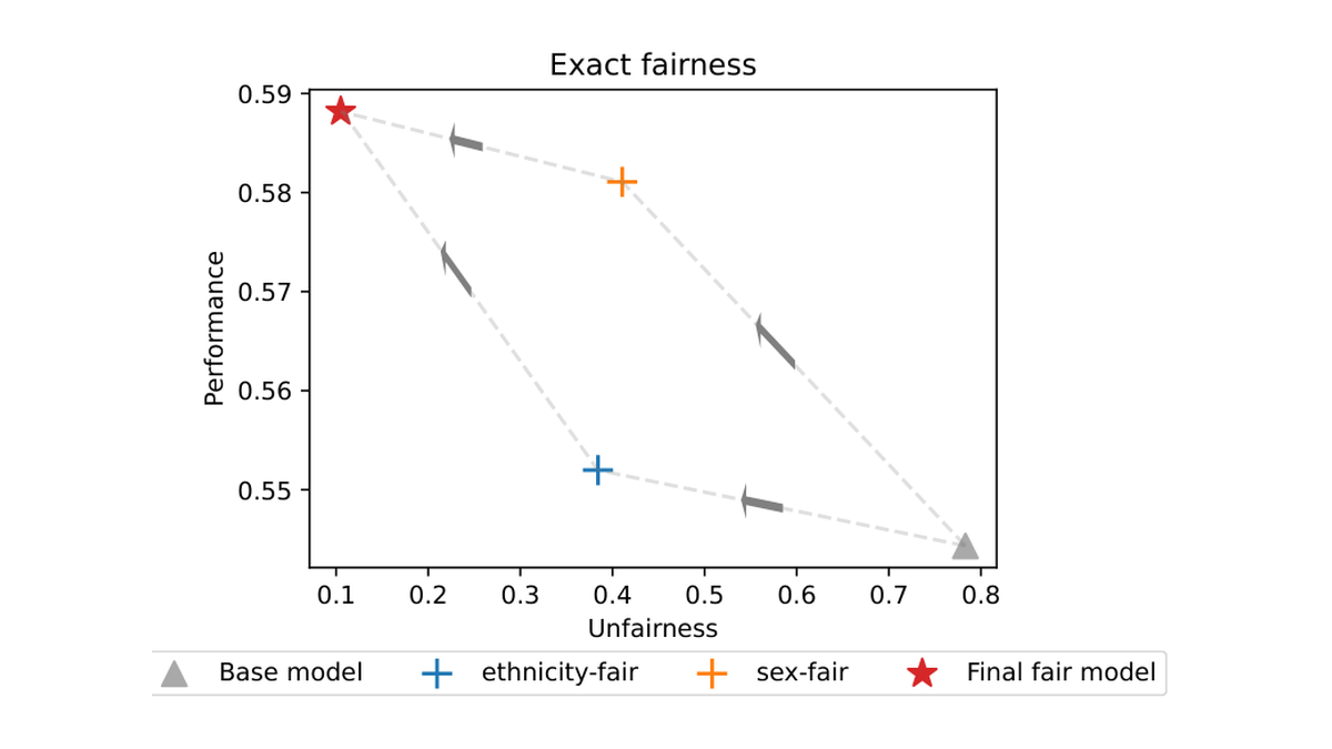
Most fairness tooling asks you to retrain. That is a reasonable thing to ask of a research prototype and an unreasonable thing to ask of a production model, which has been validated, documented, signed off, and in insurance sometimes filed with a regulator. Occasionally you cannot retrain even in principle, because the model arrives as a vendor’s binary and all you get is a column of scores.
EquiPy is built for that situation. It sits after the model, takes the scores it already produces plus the sensitive attributes, and returns corrected scores. It never sees the model, and it never sees the labels.
That last point is worth pausing on, because it is what separates EquiPy from FairLearn’s post-processing and from OxonFair: both need the outcome variable to calibrate. EquiPy calibrates on predictions and sensitive attributes alone, which is exactly what a deployment pipeline usually has lying around.
What it corrects towards
The fairness criterion is Demographic Parity: the distribution of scores should not depend on the sensitive attribute. Note that this is a statement about distributions, not about direct effects. Dropping the sensitive column does not achieve it, because a model with enough features will happily reconstruct the variable from proxies. Height correlates with sex, so a model using height is using sex.
The correction is optimal transport. Take the score distributions of each group, find the Wasserstein barycenter, which is the distribution sitting between them that costs the least to reach, and transport every group’s scores onto it. The barycenter is not an arbitrary choice of middle ground: among all distributions satisfying Demographic Parity, it is the one that moves the original predictions least, and since every movement away from the original scores costs accuracy, least movement means least damage.
In code that is two methods, deliberately shaped like scikit-learn:
from equipy.fairness import FairWasserstein

calibrator = FairWasserstein(sigma=0.0001)
calibrator.fit(predictions_calib, sensitive_feature_calib)
calibrator.transform(predictions_test, sensitive_feature_test)
sigma is jittering: a small amount of noise that breaks up atoms in the score
distribution, which the transport step needs in order to be well defined.
Several attributes at once
This is the part the package exists for. Age, sex and origin are not corrected independently, because correcting one shifts the others, and naive sequential correction quietly undoes itself.
MultiWasserstein implements the sequential mechanism from our AAAI 2024 paper.
The overall fair predictor decomposes into a composition of single-attribute
corrections:
and the destination does not depend on the order. Correcting for origin then sex lands in the same place as sex then origin. The API is identical to the single-attribute case, with a dataframe of sensitive columns instead of one:
from equipy.fairness import MultiWasserstein

calibrator = MultiWasserstein(sigma=0.0001)
calibrator.fit(predictions_calib, sensitive_features_calib)
calibrator.transform(predictions_test, sensitive_features_test)
Because the destination is fixed, the route becomes something you can study rather than something you have to worry about, and that is where the graphics come in.
Watching the trade-off
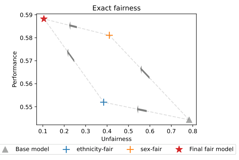
Figure 6 from the paper. The base model is bottom right: most unfair, lowest error. Each correction moves left, reducing unfairness, and up, raising mean squared error. Both routes end on the same red star.
The arrow plot is the picture I reach for in front of a risk committee, because it puts the price of fairness on an axis. Two things are visible at once. The destination is the same whichever order you choose, which is the theorem. And the routes are not the same: correcting for sex first costs noticeably more accuracy for the same reduction in unfairness. A committee choosing a correction order is making a real decision, and this plot is what makes it an explicit one rather than an implicit one. The paper connects that to fairwashing, the practice of picking whichever correction story flatters the model most.
Partial correction
Full fairness is not always the goal, or the legal requirement. EquiPy takes a vector \(\varepsilon\) giving, per attribute, how much of the available unfairness reduction to actually apply:
calibrator.transform(predictions_test, sensitive_features_test,
                     epsilon=[0.5, 0.25])
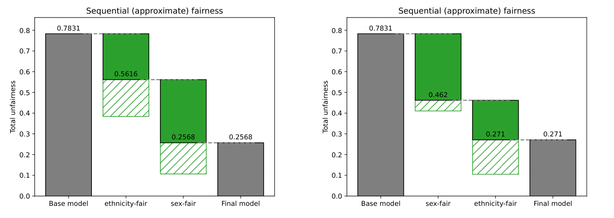
Figure 7 from the paper. Total unfairness falls from 0.78 to roughly 0.26, step by step, under both correction orders.
The waterfall plot reads left to right as a budget: each bar is one attribute’s contribution to the reduction. Correcting ethnicity first at 50% removes 28% of total unfairness; doing it second at the same 50% removes 24%. The endpoints under partial correction come out close but not identical, which is not a bug in the theorem. Order-independence holds for exact fairness. Once you correct each variable only partly, and the variables correlate, what is left for the second step depends on what the first step did.
Does it work
On US Census income data (the ACSIncome task from Folktables, with a LightGBM
base model), unfairness across ethnicity and sex together goes from 0.7831 to
0.1064. The per-attribute decomposition is the more interesting table:
| ethnicity | sex | both | |
|---|---|---|---|
| Base model | 0.4366 | 0.3465 | 0.7831 |
| after correcting ethnicity | 0.0466 | 0.3376 | 0.3842 |
| after correcting both | 0.0726 | 0.0338 | 0.1064 |
Read the middle row carefully. Correcting ethnicity took its unfairness from 0.44 to 0.05 and left sex almost untouched, as it should. Then read the last row: correcting sex pushed ethnicity’s unfairness back up slightly, from 0.05 to 0.07. That is the interaction the sequential framing is designed to make visible, and it is the reason a single aggregate fairness number is not enough to know what your correction did.
What it does not do
It corrects for Demographic Parity, not equalized odds, which is a deliberate restriction: DP is one of the few criteria that applies to regression and classification alike. Sensitive attributes have to be discrete. And you need a calibration set, ideally separate from training, though it can be unlabelled, which is usually the easy part.
None of that makes it a substitute for asking whether the model should exist. It makes the cost of the answer measurable.
Further reading. The software paper,
EquiPy: Sequential Fairness using Optimal Transport in Python,
with Agathe Fernandes Machado, Suzie Grondin, Philipp Ratz and Arthur
Charpentier. The theory behind the sequential mechanism is in
this post
and the AAAI 2024 paper. The package lives
on GitHub with
documentation, and installs with
pip install equipy. Figures 6 and 7 are reproduced from the software paper.