Blog NLP & LLMs · Machine learning 5 min read
Recurrent networks, animated
Three animations of the same small network: reading a sequence forward, being trained backwards through time, and reading from both ends at once. Each one makes a point the equations state but do not show.
Made in October 2020 for the NLP sessions of the Data Science pour l’Actuaire course at the Institut des Actuaires. Left online because the pictures have not aged, even if the frameworks around them have.
Recurrent networks are usually taught with an unrolled diagram and a recurrence relation, and students nod along. Then they write a training loop and discover they never understood which parts move and which parts stay still. These three animations exist because a still diagram cannot show that, and the three questions they answer are the ones that came up every year: what does the network actually do with a sequence, why does training it get harder the longer the sequence gets, and what do you buy by reading the sequence backwards as well.
1. The forward pass
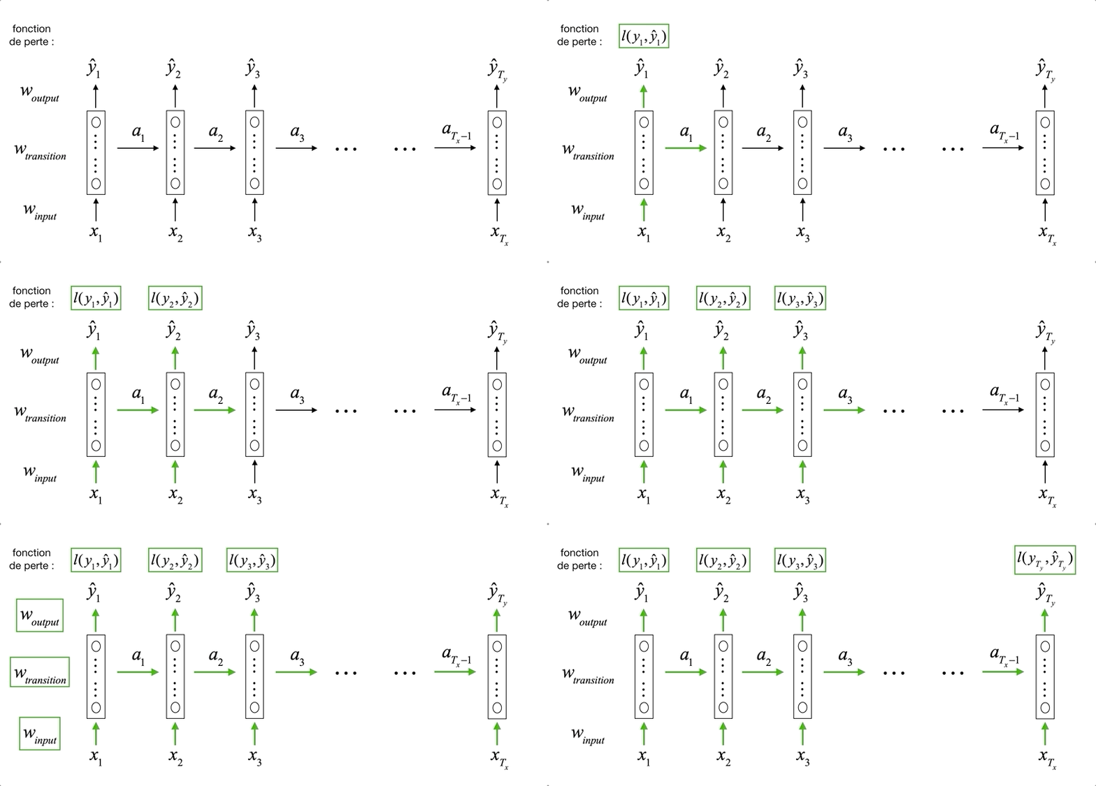
A recurrent network reads a sequence one element at a time. At step \(t\) it takes the current input \(x_t\) and the hidden state \(h_{t-1}\) left over from the previous step, and produces a new hidden state:
\[h_t = \tanh(W_x x_t + W_h h_{t-1} + b)\]That is the entire idea. The hidden state is the network’s only memory of everything it has read so far, and it is a fixed-size vector. That is both why RNNs handle sequences of any length and why they forget: everything from step 1 to step \(t\) has to be squeezed into the same few hundred numbers, and something has to give.
The part worth watching in the animation is the weights. \(W_x\) and \(W_h\) do not change as the animation moves right. The same matrices are applied at every step, which is the single most misread property of the diagram. An unrolled RNN looks like a deep network, but it is one small network applied repeatedly. That weight sharing is what makes the parameter count independent of sequence length, and it is also what makes training misbehave, which is the next animation.
2. Backpropagation through time
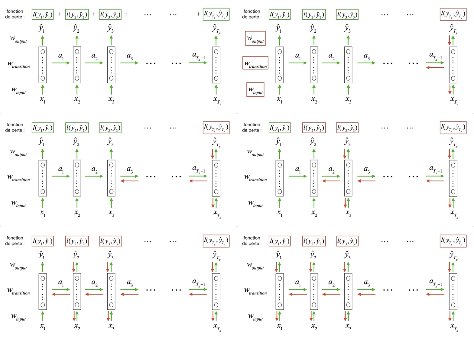
Once an RNN is unrolled, it is an ordinary feedforward network with shared weights, so it is trained by ordinary backpropagation. The only twist is bookkeeping: the loss at step \(T\) depends on \(h_{T-1}\), which depends on \(h_{T-2}\), and so on back to the beginning. Every gradient has to travel the whole chain, which is why the algorithm gets its own name.
The consequence is visible in the animation, where the red arrows walk backwards through every step the green ones walked forwards. Going from step \(T\) back to step \(k\), the gradient picks up one factor per step:
\[\frac{\partial h_T}{\partial h_k} = \prod_{t=k+1}^{T} \frac{\partial h_t}{\partial h_{t-1}}\]A product of \(T-k\) similar terms has two stable behaviours and no third one. If the factors are slightly below one, the gradient decays to nothing and the network never learns long-range dependencies. Slightly above one and it explodes. Gradient clipping handles the explosion. The vanishing case is harder, and it is the reason LSTMs and GRUs exist: they add a path along which the gradient is multiplied by something much closer to one.
Two practical notes that always come up in class. This is why people truncate backpropagation to a window of a few dozen steps rather than the full sequence. And it is why the whole forward pass has to be held in memory before any of it can be undone, which is the real reason long sequences hurt on a small GPU.
3. Reading from both ends
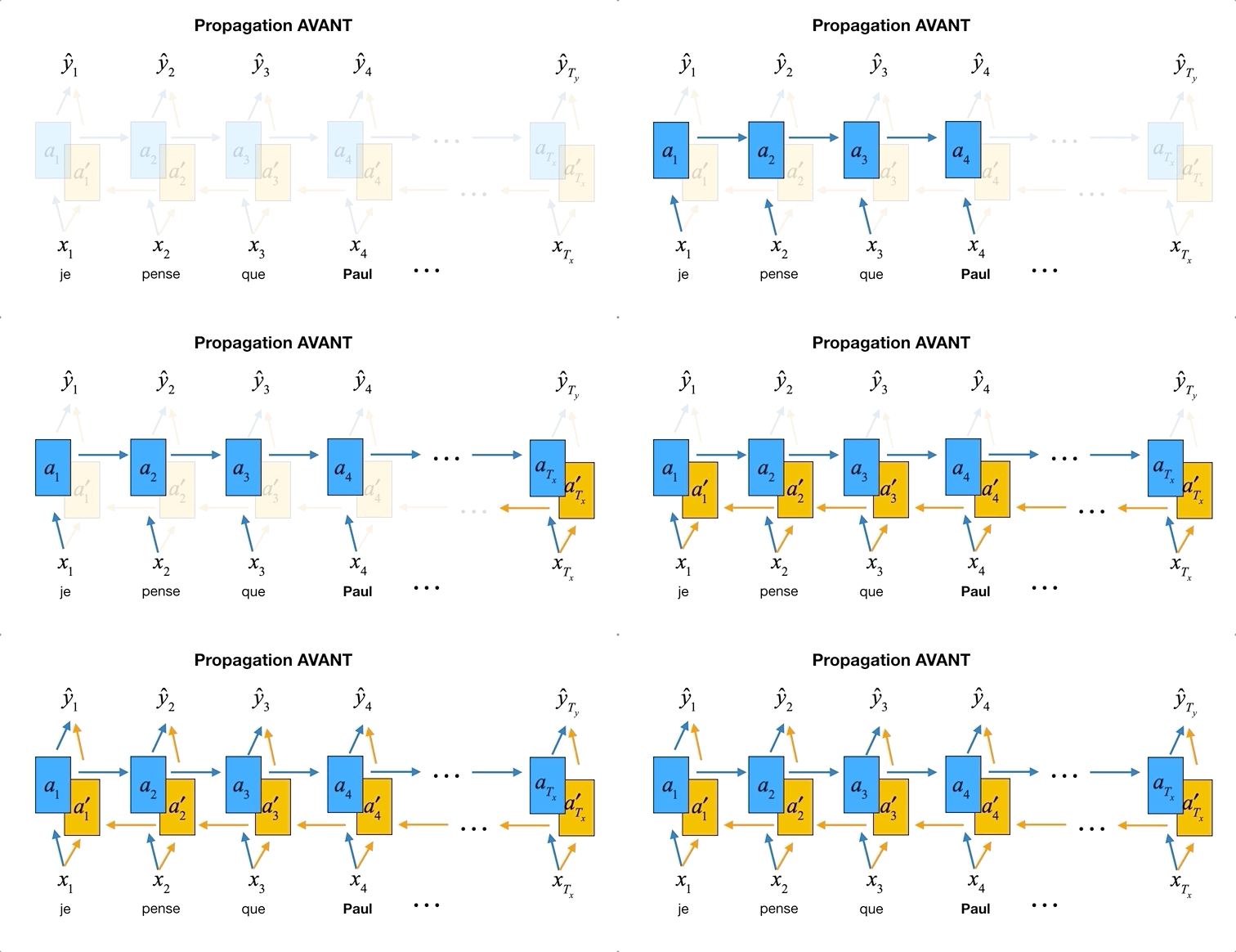
A plain RNN reading left to right knows everything before position \(t\) and nothing after it. For most language tasks that is the wrong constraint: whether bank means a riverside or a branch office is usually settled by a word further along the sentence.
A bidirectional RNN runs two independent recurrent layers over the same input, one left to right and one right to left, then glues their states together at each position:
\[h_t = [\,\overrightarrow{h_t} \; ; \; \overleftarrow{h_t}\,]\]That is the whole construction. The two directions share no weights and never talk to each other during the pass. They only meet in the concatenation, which is then what the output layer sees. In the animation the blue cells run one way, the orange cells the other, and every position ends up holding one of each.
The animation also makes the real cost obvious: the backward pass cannot start until the last element has arrived. A bidirectional model therefore needs the complete sequence up front, which rules it out for anything streaming (live transcription, real-time scoring) and is fine for anything where you already hold the whole document. That trade is the same one BERT makes and GPT does not, which is a useful thing to have seen before meeting either.
What happened next
These animations date from 2020, and the architecture they describe was already being displaced by attention when I drew them. That has not made them useless. The three ideas underneath survived the move: a hidden state as a lossy summary of everything read so far, gradients that degrade with distance, and the bidirectional trade between context and latency. Every one of those reappears, in different clothing, in the models that replaced RNNs.
The original notebook exports, if you want the raw versions: forward, backprop, bidirectional.