Blog Machine learning 2 min read
Backpropagation through time, animated
The same picture as the forward pass, run backwards. Watching the gradient travel back through every step is the fastest way to understand why long sequences are hard.
Made in October 2020 for the NLP sessions of the Data Science pour l’Actuaire course at the Institut des Actuaires. Left online because the picture has not aged, even if the frameworks around it have.
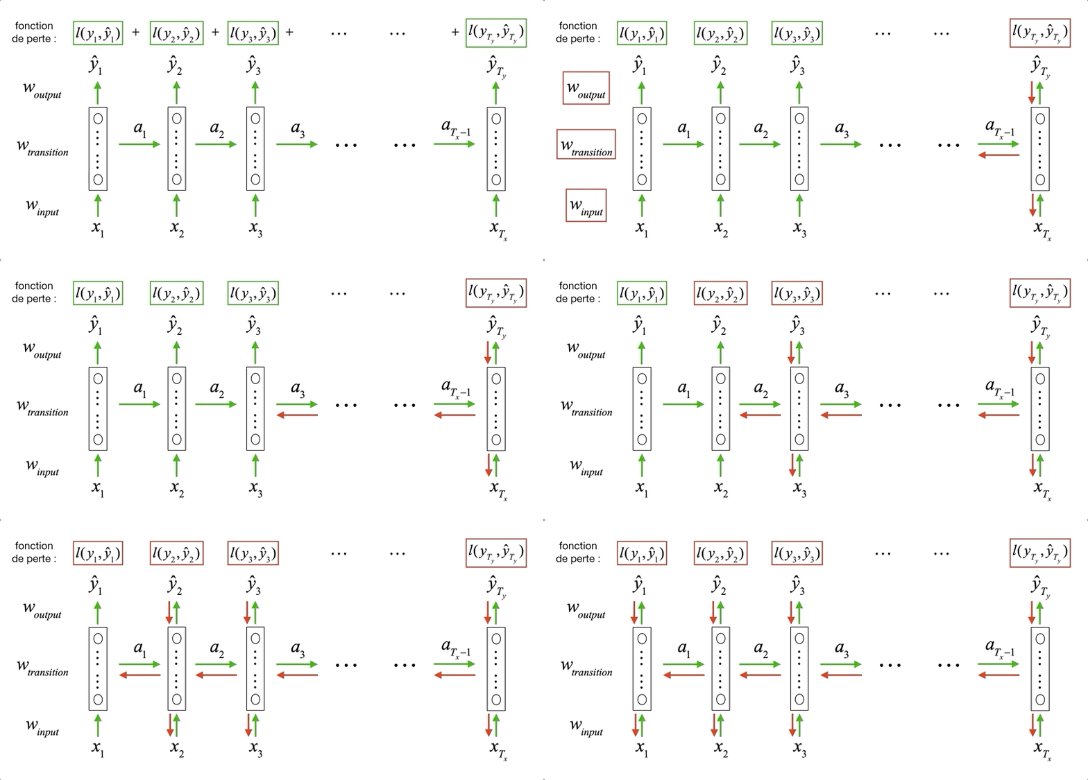
Once an RNN is unrolled, it is an ordinary feedforward network with shared weights, so it is trained by ordinary backpropagation. The only twist is bookkeeping: the loss at step \(T\) depends on \(h_{T-1}\), which depends on \(h_{T-2}\), and so on back to the beginning. Every gradient has to travel the whole chain, which is why the algorithm gets its own name.
The consequence is visible in the animation. Going from step \(T\) back to step \(k\), the gradient picks up one factor of \(W_h\) per step:
\[\frac{\partial h_T}{\partial h_k} = \prod_{t=k+1}^{T} \frac{\partial h_t}{\partial h_{t-1}}\]A product of \(T-k\) similar terms has two stable behaviours and no third one. If the factors are slightly below one, the gradient decays to nothing and the network never learns long-range dependencies; slightly above one, it explodes. Gradient clipping handles the explosion. The vanishing case is harder, and it is the reason LSTMs and GRUs exist: they add a path along which the gradient is multiplied by something much closer to one.
Two practical notes that always come up in class: this is why people truncate backpropagation to a window of a few dozen steps rather than the full sequence, and why the whole forward pass has to be kept in memory before any of it can be undone.
The original notebook export: RNN backprop. Start with the forward pass if this one is running backwards through something you have not seen yet.